Standard qSIP EAF Workflow

library(dplyr)
library(ggplot2)
library(qSIP2)
packageVersion("qSIP2")
#> [1] '0.23.0'

Background

A complete quantitative stable isotope probing (qSIP) workflow using the qSIP2 package starts with three input files and ends with calculated excess atom fraction (EAF) values along with a ton of intermediate data. This vignette will be a high-level walk through of the major steps with links to more specific vignettes where more detail is appropriate.

The Input Files

Preparing and formatting the input files is often the most tedious part of any analysis. Our goal with the rigid (and opinionated) requirements imposed by qSIP2 will hopefully streamline the creation of these files, and automated validation checks can remove many of the common sources of error or confusion. Where appropriate, qSIP2 and this documentation uses MISIP terminology¹.

Source Data

The source data is the highest level of metadata with a row corresponding to each original experimental or source material object. An example source dataframe is included in the qSIP2 package called example_source_df.

Table 1: The first few rows of example_source_df

source	total_copies_per_g	total_dna	Isotope	Moisture	isotopolog
S149	34838665	74.46539	12C	Normal	glucose
S150	53528072	109.01522	12C	Normal	glucose
S151	95774992	182.16852	12C	Normal	glucose
S152	9126192	23.68963	12C	Normal	glucose
S161	41744046	67.62552	12C	Drought	glucose
S162	49402713	94.21217	12C	Drought	glucose

There are a few required columns for valid source data including a unique ID (source_mat_id), an isotope and isotopolog designation for the substrate that had the label. Additional columns can be added as necessary (e.g. Moisture) for grouping and filtering later in the process.

For growth calculations there are three additional requirements: timepoint, total_abundance and volume. These are not necessary for the standard EAF workflow and will instead be addressed in the growth vignette.

Once the dataframe is ready, the next step is to convert it to a qsip_source_data object. This is one of the main qSIP2 objects to hold and validate the data. Each of the required columns of metadata is assigned to a column in your dataframe. For example, below the “Isotope” column in the dataframe is assigned to the isotope parameter in the qsip_source_data object.

source_object <- qsip_source_data(example_source_df,
  isotope = "Isotope",
  isotopolog = "isotopolog",
  source_mat_id = "source"
)

class(source_object)
#> [1] "qSIP2::qsip_source_data" "S7_object"

This object modifies some of the column names to standard names as supplied in the above function.

Original Headers	Modified Headers
source	source_mat_id
total_copies_per_g	total_copies_per_g
total_dna	total_dna
Isotope	isotope
Moisture	Moisture
isotopolog	isotopolog

If the column names in the dataframe already match the expected standard names, then you can skip assigning them and they should be identified correctly.

A dataframe with the original headers can be recovered using the get_dataframe() method with the original_headers = T option.

df <- get_dataframe(source_object, original_headers = TRUE)

Isotope	isotopolog	source	total_copies_per_g	total_dna	Moisture
12C	glucose	S149	34838665	74.46539	Normal
12C	glucose	S150	53528072	109.01522	Normal
12C	glucose	S151	95774992	182.16852	Normal
12C	glucose	S152	9126192	23.68963	Normal
12C	glucose	S161	41744046	67.62552	Drought
12C	glucose	S162	49402713	94.21217	Drought

See the source data vignette for more details.

Sample Data

The sample metadata is the next level of detail with one row for each fraction, or one row for each set of fastq files that were sequenced. If you have “bulk” or unfractionated sequenced reads, these are also considered samples. Basically, anything that lives as columns in your ASV/feature table are considered samples.

Table 2: The first few rows of example_sample_df

sample	source	Fraction	density_g_ml	dna_conc	avg_16S_g_soil
149_F1	S149	1	1.778855	0.0000000	4473.7081
149_F2	S149	2	1.773391	0.0000000	986.6581
149_F3	S149	3	1.765742	0.0000000	4002.7026
149_F4	S149	4	1.759185	0.0000000	3959.7283
149_F5	S149	5	1.752629	0.0012413	5725.7319
149_F6	S149	6	1.746072	0.0128156	7566.2722

Again, there are several necessary columns for valid sample data, including a unique sample ID (sample_id), the source they came from (source_mat_id), the fraction ID (gradient_position), the fraction density (gradient_pos_density) and a measure of abundance (total DNA or qPCR copy number) in that fraction (gradient_pos_amt).

An additional column that can be derived is the percent abundance of your total sample that is found in each of the fractions. The add_gradient_pos_rel_amt() function can help calculate that by dividing each fraction abundance by the total abundance for each source and putting it in a gradient_pos_rel_amt column.

But there is no need to do this if you already have the relative amounts calculated in your dataframe.

sample_df <- example_sample_df |>
  add_gradient_pos_rel_amt(source_mat_id = "source", amt = "avg_16S_g_soil")

Table 3: Additional gradient_pos_rel_amt column added

sample	source	Fraction	density_g_ml	dna_conc	avg_16S_g_soil	gradient_pos_rel_amt
149_F1	S149	1	1.778855	0.0000000	4473.7081	0.0001284
149_F2	S149	2	1.773391	0.0000000	986.6581	0.0000283
149_F3	S149	3	1.765742	0.0000000	4002.7026	0.0001149
149_F4	S149	4	1.759185	0.0000000	3959.7283	0.0001137
149_F5	S149	5	1.752629	0.0012413	5725.7319	0.0001643
149_F6	S149	6	1.746072	0.0128156	7566.2722	0.0002172

Again, we make a qSIP2 object for this data, this time as a qsip_sample_data object. The columns in the dataframe are assigned to the appropriate parameters, and any column names exactly matching the parameter name will automatically be identified. Similar to the source_data above, the names in the sample_data object will be modified from the original names to the standardized names.

sample_object <- qsip_sample_data(sample_df,
  sample_id = "sample",
  source_mat_id = "source",
  gradient_position = "Fraction",
  gradient_pos_density = "density_g_ml",
  gradient_pos_amt = "avg_16S_g_soil",
  gradient_pos_rel_amt = "gradient_pos_rel_amt"
)

class(sample_object)
#> [1] "qSIP2::qsip_sample_data" "S7_object"

See the sample data vignette for more information including the built-in validations.

Feature Data

Finally, the last of the three necessary input files is a feature abundance table, aka “OTU table” or “ASV table”. The format of this dataframe has the unique feature IDs in the first column, and an additional column for each sample. Each row then contains the whole number (non-normalized) counts of each feature in each sample. If your features are MAGs, then you may instead of coverages or some other pre-normalized value in your feature table instead of sequence counts.

For now, the validation step defaults to requiring all values be counts (positive integers), but other type options include coverage (for working with MAGs or metagenomes), relative if you already have relative abundances and normalized if you have spike-ins or another method that determines the correct abundance in each sample.

Table 4: First bit of example_feature_df

ASV	149_F1	149_F2	149_F3	149_F4	149_F5
ASV_1	1245	376	582	1258	692
ASV_2	1471	569	830	1373	737
ASV_3	342	152	211	389	218
ASV_4	288	119	161	294	157
ASV_5	317	108	95	292	164
ASV_6	201	73	130	250	112

feature_object <- qsip_feature_data(example_feature_df,
  feature_id = "ASV"
)

class(feature_object)
#> [1] "qSIP2::qsip_feature_data" "S7_object"

See the feature data vignette for more details.

The qsip_data Object

The qsip_data class is the main workhorse object in the qSIP2 package. It is built from validated versions of the three previous objects, and is meant to be a self-contained object with all of the necessary information for analysis.

qsip_object <- qsip_data(
  source_data = source_object,
  sample_data = sample_object,
  feature_data = feature_object
)
#> ✔ There are 15 source_mat_ids, and they are all shared between the source and sample objects.
#> ✔ There are 284 sample_ids, and they are all shared between the sample and feature objects.

class(qsip_object)
#> [1] "qSIP2::qsip_data" "S7_object"

This function will report if all source_mat_ids are shared between the source and sample data, and if all sample_ids are shared between the sample and feature data. If it reports there are some unshared ids, you can access them with get_unshared_ids(qsip_object), but note that it is just a warning and does not stop the creation of the qSIP object.

Visualizations

Behind the scenes, creation of this object also runs some other calculations, particularly getting the weighted-average density (WAD) for each feature in each source, and also the tube relative abundance of each feature. With these, certain visualizations can be made with built-in functions.

plot_source_wads(qsip_object, 
                 group = "Moisture")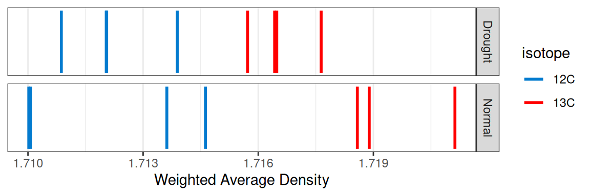

Figure 1: WAD of each source, grouped by Moisture. Note that for this example dataset the 13C just happens to have source-level WAD values greater than the 12C, but it is generally not a concern if the 12C and 13C values are intermingled.

plot_sample_curves(qsip_object,
                   facet_by = "isotope",
                   show_wad = F)

Figu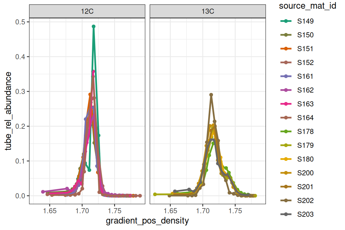re 2: Normalized density curves for each source_mat_id. The y-axis is scaled to tube fraction abundance.

Another sanity check is making sure the reported density values are on a reasonably straight line with the gradient position with a Cook’s distance to highlight any outliers in red. Note, the ends of the gradient are often flagged as outliers, although this may not necessarily be the case.

plot_density_outliers(qsip_object)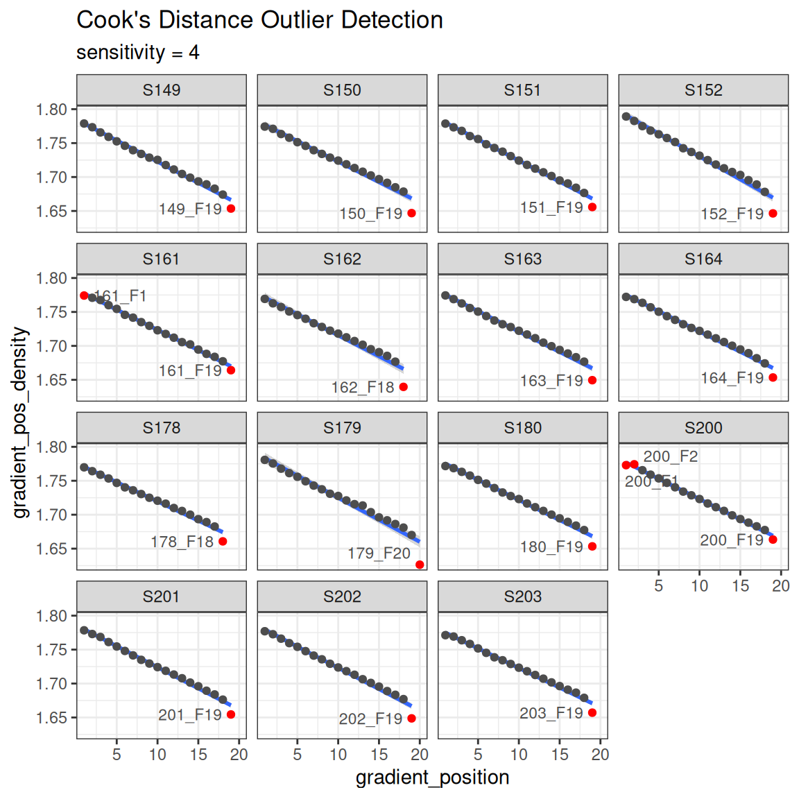

Figure 3

An important note about qsip_data objects

The design of the qsip_data object is that it is contains “slots” for each new analysis step. Although you could create a new object for each step of the workflow, you can assign the output of each step back to the original object in order to keep everything together. “Printing” the qsip_data object will give some summary data as well as TRUE/FALSE flags for which steps have been done on that object.

print(qsip_object)
#> <qsip_data>
#> group: none
#> feature_id count: 2030 of 2030
#> sample_id count: 284
#> filtered: FALSE
#> resampled: FALSE
#> EAF: FALSE
#> growth: FALSE

Main Workflow

Now that we have a validated qsip_data object, we can start the main workflow consisting of comparison grouping, filtering, resampling and finally calculating EAF values. Note that this workflow explicitly (and laboriously) runs through all of the steps individually, but the preferred workflow is either piping them all together, or ideally running the multiple objects workflow. Both of these are previewed below with links to the full vignette.

Comparison Grouping

Your qsip_data object likely contains all of your data, but you may only want to run comparisons on certain subsets. The get_comparison_groups() function attempts to identify and suggest the sources you may want to compare.

Table 5: Output of get_comparison_groups().

get_comparison_groups(qsip_object,
  group = "Moisture",
  isotope = "isotope",
  source_mat_id = "source_mat_id"
)
#> # A tibble: 2 × 3
#>   Moisture `12C`                  `13C`                 
#>   <chr>    <chr>                  <chr>                 
#> 1 Normal   S149, S150, S151, S152 S178, S179, S180      
#> 2 Drought  S161, S162, S163, S164 S200, S201, S202, S203

The group argument here is the most important as it will define the rows that it thinks constitute a comparison. If you have more complicated groupings that involve multiple columns of metadata, you can instead run a paste call inside mutate to create combined column:

qsip_object |>
  mutate(new_column = paste(column1, column2, sep = "_")) |>
  get_comparison_groups(
    group = "new_column",
    isotope = "isotope",
    source_mat_id = "source_mat_id"
  )

The isotope argument is what defines the labeled and unlabeled values for the comparisons. This can be more complex, particularly if you have more than one isotopolog. For example, a study with some 13C sources, other 15N sources, and a shared 12C/14N natural abundance source material. Please reach out via qSIP2 github issues for more complex study designs.

The first row shows what “Normal” moisture groups we likely want to use for unlabeled (S149, S150, S151 and S152) to compare to the labeled (S178, S179 and S180). Sometimes you may also want to compare the specific labeled samples in a group to all unlabeled. The qSIP2 package has a convenient way to get those by using the get_all_by_isotope() function.

get_all_by_isotope(qsip_object, "12C")
#> [1] "S149" "S150" "S151" "S152" "S161" "S162" "S163" "S164"

The get_comparison_groups() function is entirely informational, but it is possible to pipe this output into the run_comparison_groups() function. This more advanced use in detailed in the Multiple qSIP Objects vignette.

Filter Features

The filter features step does two things. First, it is where the set of labeled and unlabeled sources are defined for a specific comparison. Second, it is where you can explicitly say how prevalent a feature must be to be considered “present” in a source. In other words, you define the parameters that a feature must be found enough of the replicate sources, and in enough samples that you can calculate an accurate WAD value for it.

The run_feature_filter() function takes a qsip_data object and these different parameters allowing you to precisely tailor your filtering results. The more strict the filtering, the fewer features that will pass the filter.

qsip_normal <- run_feature_filter(qsip_object,
  unlabeled_source_mat_ids = get_all_by_isotope(qsip_object, "12C"),
  labeled_source_mat_ids = c("S178", "S179", "S180"),
  min_unlabeled_sources = 6,
  min_labeled_sources = 3,
  min_unlabeled_fractions = 6,
  min_labeled_fractions = 6,
  quiet = TRUE
)

Note, although I said earlier you can overwrite your qsip_data objects as you go, here it might make sense to create two versions for the moisture treatments. We’ll take the original qsip_object and save the filtered Normal dataset to qsip_normal', and the Drought toqsip_drought`.

Of the 1,705 features found in the “Normal” data, we can see our rather strict filtering removed all but 64 features from the dataset.

df = get_filter_results(qsip_normal)

Table 6: Detailed results of the filtering.

filter_step	features_unlabeled	features_labeled	union	intersect	unlabeled_only	labeled_only	mean_abundance_unlabeled	mean_abundance_labeled
Zero Fractions	1519	1417	1560	1376	143	41	0.0000000	0.0000000
Fraction Filtered	1440	830	1646	624	816	206	0.1579295	0.2053189
Fraction Passed	299	209	346	162	137	47	0.8420705	0.7946811
Zero Sources	47	137	184	0	47	137	0.0000000	0.0000000
Source Filtered	196	127	265	58	138	69	0.3167506	0.2163507
Source Passed	103	82	121	64	39	18	0.7631509	0.6849542

We can visualize these results on a per-source basis with the plot_filter_results() function.

plot_filter_results(qsip_normal)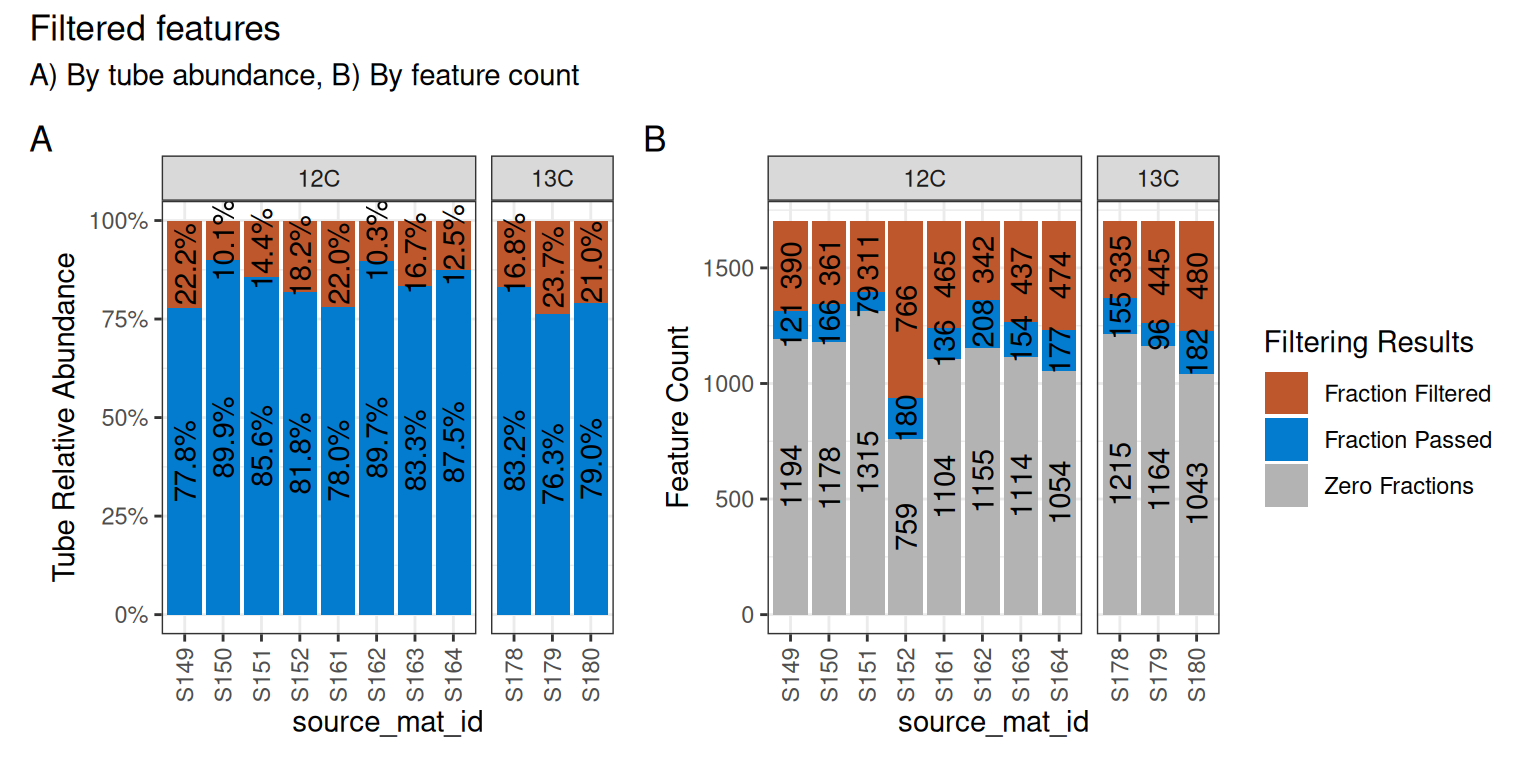

Figure 4: Per-source filtering results for the “normal” dataset.

Although a large number of features were removed, we can tell that the 64 that remained actually still make up a large proportion of the total abundance in each sample. In A above, the retained features (in blue) make up ~75-85% of the total data, while the removed data (orange) is the remaining ~15-25%.

In B, we can see that a surprisingly large number of features are found 0 times in many sources (gray) and will therefore never be present regardless of our filtering choices. And although there are are ~100-200 features that passed the filtering requirements (blue), our requirement that min_unlabeled_sources = 6 and min_labeled_sources = 3 means that only the features present in many of the blue slices will be retained, leaving only 64 total.

Let’s do the same comparison with the drought samples.

qsip_drought <- run_feature_filter(qsip_object,
  unlabeled_source_mat_ids = get_all_by_isotope(qsip_object, "12C"),
  labeled_source_mat_ids = c("S200", "S201", "S202", "S203"),
  min_unlabeled_sources = 6,
  min_labeled_sources = 3,
  min_unlabeled_fractions = 6,
  min_labeled_fractions = 6,
  quiet = TRUE
)

And only 89 features were retained in the Drought dataset.

plot_filter_results(qsip_drought)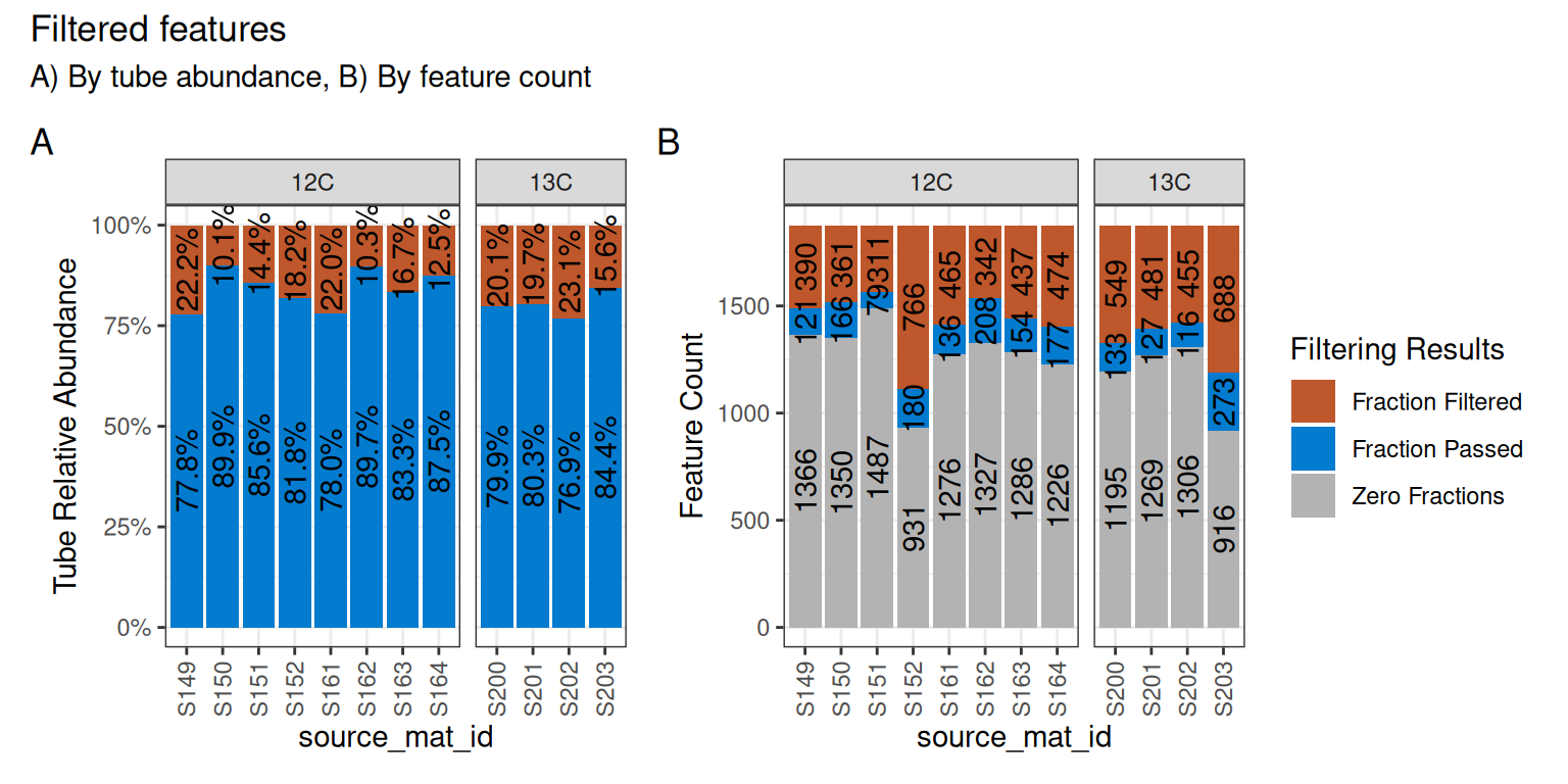

Figure 5: Per-source filtering results for the “drought” dataset.

Strictly speaking, there is no requirement to do strict filtering, and it is possible to execute run_feature_filter() with all parameters set to 1. Filtering was originally recommended because it dramatically sped up the compute time, but running all vs. a subset of features in qSIP2 has a minimal impact. Further, setting all values to 1 and utilizing the allow_failures flag in the resampling step can provide an alternative way of deciding which features to keep, rather than just their prevalence amongst sources/samples. More information is provided in the resampling section below, or the resampling vignette.

Importantly, since the relative abundances have already been calculated for each feature, the subsequent steps in the qSIP pipeline keep each feature’s computations independent, and the results for a specific feature will be identical regardless of whether other features are included or filtered out.

Resampling

The weighted average density (WAD) values were automatically calculated during the creation of the qsip_data object earlier. In order to calculate the confidence interval for the EAF values, we first need to run a resampling/bootstrapping procedure on the WAD values. For example, a feature found in 6 unlabeled sources will have 6 WAD values, and these 6 WAD values are resampled many times to obtain bootstrapped mean WAD values.

qsip_normal <- run_resampling(qsip_normal,
  resamples = 1000,
  with_seed = 17,
  progress = FALSE
)

As this step requires some random sampling it is good practice to set the “seed”. Rather than doing this outside of the function, you can pass the seed as an argument. If you leave blank, it will generate a random seed. The seed will generate the same results each time you run the resampling process.

qsip_normal_17_again <- run_resampling(qsip_normal,
  resamples = 1000,
  with_seed = 17,
  progress = FALSE
)

# two runs are identical
identical(qsip_normal, qsip_normal_17_again)
#> [1] TRUE
identical(qsip_normal@resamples$l[[334]], qsip_normal_17_again@resamples$l[[334]])
#> [1] TRUE

# but individual resamplings within are different
identical(qsip_normal@resamples$l[[1]], qsip_normal@resamples$l[[2]])
#> [1] FALSE

Ressampling of the drought dataset. Notice at this step we are overwriting the original qsip_drought with the results of run_resampling(), rather than creating new objects.

qsip_drought <- run_resampling(qsip_drought,
  resamples = 1000,
  with_seed = 17,
  progress = FALSE
)

It is possible to get a resampling error if your filtering is too strict. If so, consult the resampling vignette and consider running with allow_failures = T.

EAF Calculations

And we are finally at the last main step, calculating and summarizing the excess atom fraction (EAF) values. There are two functions to run, the first (run_EAF_calculations()) that calculate EAF for the observed data and all resamplings, and the second (summarize_EAF_values()) that summarizes that data at a chosen confidence interval. These are split into two functions simply because the run_EAF_calculations() can take a little longer, allowing different parameters to be tried in summarize_EAF_values() without having to recalculate everything. More more information see the EAF vignette.

We’ll also mutate() to add the original Moisture condition to each dataframe before we combine them. Note, there is a better way to run and get results with multiple qSIP2 objects - more details below.

qsip_normal <- run_EAF_calculations(qsip_normal)
qsip_drought <- run_EAF_calculations(qsip_drought)

normal <- summarize_EAF_values(qsip_normal, confidence = 0.95) |>
  mutate(Moisture = "Normal")
#> Confidence level = 0.95

drought <- summarize_EAF_values(qsip_drought, confidence = 0.95) |>
  mutate(Moisture = "Drought")
#> Confidence level = 0.95

eaf <- rbind(normal, drought)

We can plot the top 50 by each moisture condition.

plot_EAF_values(qsip_normal, 
                top = 50, 
                confidence = 0.95, 
                error = "ribbon")
#> Confidence level = 0.95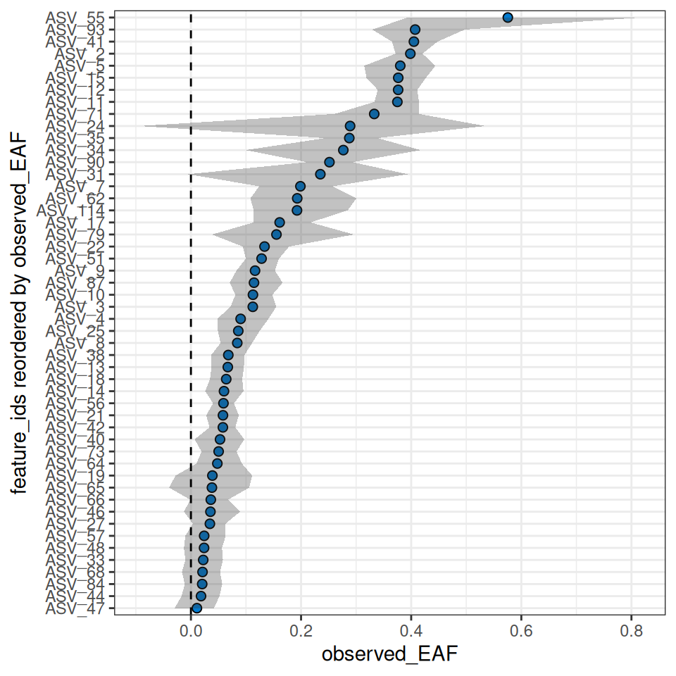

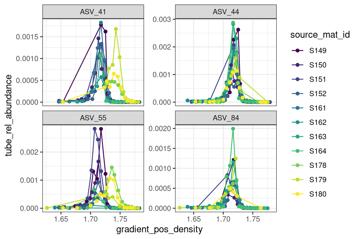
Figure 6: EAF of the top 50 features in the Normal moisture dataset

The plot_feature_curves() function allows us to plot the tube relative abundances for specific feature IDs. Let’s look at two with high EAF values, and two with low values.

plot_feature_curves(qsip_normal,
  feature_ids = c("ASV_55", "ASV_84", "ASV_41", "ASV_44")
)

Figure 7: Density curves of selected features

Delta EAF

To determine if there are any differences in how a feature responds in different treatments, we can run the delta EAF workflow. This workflow is detailed in the delta EAF vignette.

The trick is to make a list() of multiple objects with a name that reflects their grouping.

qsip_list = list("Normal" = qsip_normal,
                 "Drought" = qsip_drought)

Then, the run_delta_EAF_contrasts() function will infer the proper contrasts (there is only one in this case) and will assign which is the control and which is the treatment. See the vignette for more control over these decisions.

df = run_delta_EAF_contrasts(qsip_list, confidence = 0.95)
#> ℹ `contrasts` not given so running all-by-all
#> ℹ Confidence level = 0.95
#> ! there were 0 contrast and 0 bs_pval result messages

feature_id	contrast	delta	lower	upper	sd	bs_pval	bs_pval_message	pval	contrast_message
ASV_1	Drought vs Normal	0.0180749	-0.0546814	0.0969191	0.0381461	0.668	NA	0.6356180	NA
ASV_10	Drought vs Normal	0.0583124	0.0136634	0.1004436	0.0224994	0.006	NA	0.0095494	NA
ASV_11	Drought vs Normal	0.1119790	0.0375634	0.1885486	0.0385194	0.000	NA	0.0036482	NA
ASV_114	Drought vs Normal	-0.0234184	-0.1607945	0.1180637	0.0699282	0.702	NA	0.7377065	NA
ASV_12	Drought vs Normal	0.0482223	0.0031208	0.0895461	0.0225526	0.036	NA	0.0324997	NA
ASV_13	Drought vs Normal	0.0482378	0.0001856	0.0936535	0.0235292	0.048	NA	0.0403524	NA

Just looking at a few of these, the delta is the difference in EAF value for those features. Since the function “guessed” the contrasts and set as “Drought vs Normal”, this is saying “Drought” is the control, and the delta is reported as \(Normal - Drought\), so a positive number means higher in the Normal. The lower/upper values are the 95% CI of the bootstrap values, and bs_pval is the p-value under the null hypothesis that the true delta is approximately zero.

Working with multiple qSIP objects

It is possible to work with multiple qsip_data objects if they are in a list. This is detailed in the multiple objects vignette, but here is a sneak peak where we can use the existing summarize_EAF_values() or plot_EAF_values() functions.

Like above in the delta EAF section, this also involves using a list of qsip_data objects.

df = summarize_EAF_values(qsip_list) 
#> Confidence level = 0.9

group	feature_id	observed_EAF	mean_resampled_EAF	lower	upper	pval	labeled_resamples	unlabeled_resamples	labeled_sources	unlabeled_sources
Normal	ASV_1	-0.0153107	-0.0157044	-0.0516543	0.0236518	0.470	1000	1000	3	8
Drought	ASV_1	-0.0333856	-0.0330890	-0.0808509	0.0161212	0.284	1000	1000	4	8
Normal	ASV_10	0.1126260	0.1121874	0.0848992	0.1400368	0.000	1000	1000	3	8
Drought	ASV_10	0.0543136	0.0541364	0.0303215	0.0776436	0.000	1000	1000	4	8
Drought	ASV_100	-0.0892684	-0.0895131	-0.1488307	-0.0349891	0.016	1000	1000	3	7
Drought	ASV_102	-0.0407091	-0.0407609	-0.0907747	0.0088904	0.168	1000	1000	4	8
Normal	ASV_11	0.3749260	0.3743849	0.3392976	0.4094196	0.000	1000	1000	3	8
Drought	ASV_11	0.2629470	0.2622983	0.2041474	0.3099201	0.000	1000	1000	4	8
Normal	ASV_114	0.1926455	0.1918100	0.1234247	0.2683575	0.000	1000	1000	3	7
Drought	ASV_114	0.2160639	0.2167657	0.1304984	0.2998898	0.000	1000	1000	3	7

plot_EAF_values(qsip_list, 
                confidence = 0.9, 
                shared_y = TRUE,
                error = "bar")
#> Confidence level = 0.9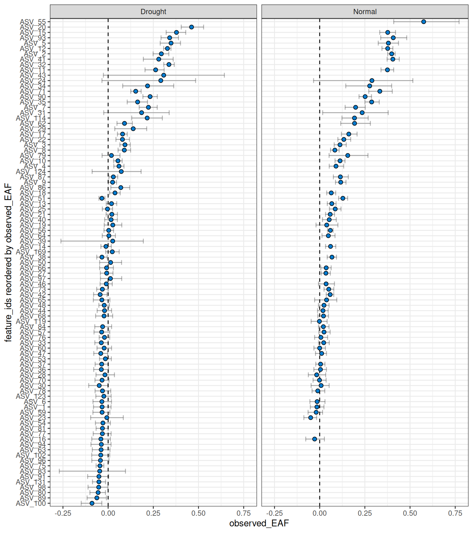

Both treatments shown together with a shared Y axis.

This version of the workflow still requires running each comparison separately. A cleaner workflow, and the recommended route, is to define your comparisons upstream, even in an Excel file, and run that dataframe through the workflow. Details can be found in the Multiple qSIP Objects vignette.

Piped Workflow

Although the workflow is often easier to understand and troubleshoot when broken into individual steps, it is possible to run the entire workflow in a single pipe.

For example, the normal moisture data could be filtered, resampled and have EAF values calculated in a single pipe.

# example code, not executed. Default values are not shown.

qsip_normal <- run_feature_filter(qsip_object,
  unlabeled_source_mat_ids = get_all_by_isotope(qsip_object, "12C"),
  labeled_source_mat_ids = c("S178", "S179", "S180"),
  min_unlabeled_sources = 6,
  min_labeled_sources = 3,
  quiet = TRUE
) |>
  run_resampling(with_seed = 44, 
                 progress = F) |>
  run_EAF_calculations()