Growth Workflow

library(dplyr)
library(ggplot2)
library(qSIP2)
packageVersion("qSIP2")
#> [1] '0.24.0'

Background

The growth workflow extends the standard qSIP approach to estimate birth and death rates of individual features over time. This vignette walks through the additional data requirements, the growth calculation procedure, and how to interpret and troubleshoot growth results. Growth analysis starts with EAF calculations, so you should be familiar with the standard qSIP workflow before proceeding.

Using qSIP2, we can estimate the growth rate of individual features (i.e. bacteria) in a microbial community by fitting a growth model to the abundance of a labeled taxon over time. Assumptions for growth include:

1. There is no isotopic labeling at time zero
2. The pool of unlabeled features will not increase over time
3. Bacteria that incorporate the isotope are 100% labeled

Using the calculated EAF values from the standard workflow, we therefore can say an EAF of 0.5 means that 50% of the bacteria are labeled and the result of growth since time zero (i.e. “birth” or \(b_i\)). Further, using quantitative abundance values in both time zero and time point samples, we can estimate the death rate (\(d_i\)) of individual features by calculating the decrease in unlabeled features. Together, we get at the growth rate using the equation \(r_i = b_i + d_i\) for each feature \(i\)¹. This is one of the main advantages of qSIP: if \(b\) equals \(d\) then traditional community analysis would detect no change in the community, whereas qSIP would detect growth and death of individual features.

For growth, three additional arguments are required for the qsip_source_data creation:

1. timepoint - a numerical value for the timepoint of the source material. There is often a 0 timepoint, but these can be any values and the growth rate will be calculated as the difference between time points. Further, these can be any units (e.g. days, hours, etc.), and the interpretation of the growth rate will depend on the units (e.g. “per day” or “per hour”).
2. total_abundance - a numerical value for the total abundance of the source material. Ideally, this is a copy number from qPCR using the same primers as the sequencing. Further, it should be standardized to some unit of starting material (e.g. copies per gram of soil). If it isn’t, then the next volume argument is important.
3. volume - a numerical value for the volume of the source material DNA that the copy number was derived from. Typically the volume is the same for all source material DNA extractions, but if your starting volume for qPCR was different then this parameter is important.

Growth Object

An example growth object is provided with the qSIP2 package called example_qsip_growth_object. Before running the workflow, it’s useful to inspect this object to understand how the additional growth-related columns are structured. We can pull out a table with the relevant columns to verify the data is formatted correctly.

get_dataframe(example_qsip_growth_object, type = "source") |> 
  select(source_mat_id, isotope, timepoint, total_abundance, volume) |>
  arrange(timepoint, isotope)

Table 1: Source data for the growth object showing timepoint, isotope, total abundance, and volume information.

source_mat_id	isotope	timepoint	total_abundance	volume
source_1	Time0	0	20934337125	1
source_10	Time0	0	56376407410	1
source_13	Time0	0	7952816086	1
source_4	Time0	0	38061061332	1
source_7	Time0	0	28775383886	1
source_11	16O	10	5053795437	1
source_14	16O	10	219349821	1
source_2	16O	10	5006451196	1
source_5	16O	10	5440927504	1
source_8	16O	10	3000381981	1
source_12	18O	10	5043787157	1
source_15	18O	10	200708494	1
source_3	18O	10	5524820407	1
source_6	18O	10	5242785770	1
source_9	18O	10	3702908766	1

From Table 1, we can notice a few things. First, there are 15 total samples - 5 with timepoint 0, and 5 each with ¹⁶O or ¹⁸O isotopes. Second, some sources do not have a standard isotope designation, but instead say “Time0”. This is a special allowed isotope type flagging these sources as unfractionated, and therefore no EAF value will be calculated for them. Third, the volume column is the same for all samples which indicates that the total_abundance is already standardized to the same volume. Indeed if we look at the column that total_abundance was derived from we can tell from the name that it is a copy number standardized to a consistent amount of soil (16S copies per gram of soil).

example_qsip_growth_object@source_data@total_abundance
#> [1] "qPCR.16S.copies.g.soil"

EAF Workflow

As mentioned above, the growth workflow requires the EAF values to be calculated first. The workflow follows the same pattern as the standard qSIP workflow: filter features, run resampling, and calculate EAF values. Note that we are running with allow_failures = TRUE, but still with a minimum of 4 labeled and 4 unlabeled fractions.

q <- run_feature_filter(example_qsip_growth_object,
  group = "Day 10",
  unlabeled_source_mat_ids = c("source_11", "source_14", "source_2", "source_5", "source_8"),
  labeled_source_mat_ids = c("source_12", "source_15", "source_3", "source_6", "source_9"),
  min_labeled_fractions = 4,
  min_unlabeled_fractions = 4
) |>
  run_resampling(
    resamples = 1000,
    with_seed = 1332,
    allow_failures = TRUE,
    progress = FALSE
  ) |>
  run_EAF_calculations()
#> There are initially 364 unique feature_ids
#> 364 of these have abundance in at least one fraction of one source_mat_id
#> =+=+=+=+=+=+=+=+=+=+=+=+=+=+=+=+=+=+=+=+=+=+=+=+=+
#> 
#> Filtering feature_ids by fraction...
#> 
#> ✖ 15 unlabeled and 11 labeled feature_ids found in zero fractions in at least
#>   one source_mat_id
#> ✖ 70 unlabeled and 47 labeled feature_ids found in too few fractions in at
#>   least one source_mat_id
#> ✔ 364 unlabeled and 364 labeled feature_ids passed the fraction filter
#> ℹ In total, 364 unique feature_ids passed the fraction filtering requirements
#> =+=+=+=+=+=+=+=+=+=+=+=+=+=+=+=+=+=+=+=+=+=+=+=+=+
#> 
#> Filtering feature_ids by source...
#> 
#> ✖ 6 unlabeled and 5 labeled feature_ids failed the source filter because they
#>   were found in too few sources
#> ✔ 358 unlabeled and 359 labeled feature_ids passed the source filter
#> ℹ In total, 358 unique feature_ids passed all fraction and source filtering
#>   requirements
#> Warning: 9 unlabeled and 6 labeled feature_ids had resampling failures.
#> ℹ Run `get_resample_counts()` or `plot_successful_resamples()` on your
#>   <qsip_data> object to inspect.

Overall, most features had robust resampling results, with only a few having less than 99% success in the labeled sources (Table 2).

Table 2: Features with fewer than 1000 successful resamples during EAF calculation.

get_resample_counts(q) |>
  filter(labeled_resamples < 1000 | unlabeled_resamples < 1000)
#> # A tibble: 11 × 3
#>    feature_id labeled_resamples unlabeled_resamples
#>    <chr>                  <int>               <int>
#>  1 taxon_113               1000                 324
#>  2 taxon_180               1000                 324
#>  3 taxon_233               1000                 336
#>  4 taxon_234                 88                  53
#>  5 taxon_245                353                1000
#>  6 taxon_250                 89                  76
#>  7 taxon_278               1000                 324
#>  8 taxon_292                307                 324
#>  9 taxon_327                353                 324
#> 10 taxon_341               1000                 324
#> 11 taxon_74                 307                1000

plot_EAF_values(q,
  confidence = 0.9,
  error = "ribbon",
  success_ratio = 0.9
)
#> ℹ Confidence level = 0.9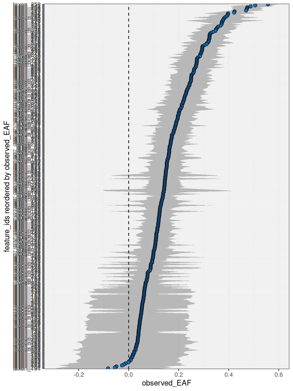

Figure 1: EAF values for Day 10 timepoint with 90% confidence intervals shown as ribbons.

Overall, most features had robust resampling results. Now that we have EAF values, we can proceed to the growth calculations.

Growth Workflow

Time zero total abundances

In addition to the EAF values stored in the qsip_data object, we also need a table with the \(N_{TOTALi0}\) values for each feature \(i\) at timepoint \(t\), in this case time 0. This value is the total abundance of each feature and is the sum of both the labeled and unlabeled features (equation 2 from Koch et al. 2018²). Note you don’t have to always compare against time zero. If you have a 7-day and 14-day timepoint you can set day 7 as the initial timepoint here.

This table is created with the get_N_total_it() function where you pass the original qsip_data object and the timepoint of interest.

Note: get_N_total_it() should be run on the initial qsip_data object before any filtering or resampling has been done. This is because the unfractionated time zero sources will not be present in the filtered data.

N_total_i0 <- get_N_total_it(example_qsip_growth_object, t = 0)
#> Warning: 1 feature_id have zero abundance at time 0: "taxon_194"

Note we get a warning here that taxon_194 has zero abundance at t = 0. Therefore, this feature cannot have a growth rate calculated because any change in abundance would be considered infinite growth. We’ll see how this is handled in the When growth cannot be calculated section below.

Table 3: First few rows of N_total_i0 showing total abundance at time zero for each feature.

feature_id	N_total_i0	timepoint1
taxon_1	1595472105	0
taxon_2	64576684	0
taxon_3	4488930	0
taxon_4	2494463	0
taxon_5	9849881	0
taxon_6	697760597	0

Growth rate calculations

Using the abundance values stored in N_total_i0 and the resampled EAF values stored in q, we can calculate the growth rate for each feature. This is done with the run_growth_calculations() function where you pass the qsip_data object, the N_total_i0 table, and the growth model to use. The growth model can be either “exponential” or “linear”.

q <- run_growth_calculations(q,
                               N_total_it = example_qsip_growth_t0,
                               growth_model = "exponential")
#> Warning: 31327 resamplings have a negative EAF value or calculated labeled copy numbers
#> less than 0. Filtered out and added to @growth$negative_labeled

Note the warning message indicating 31862 resamplings with negative EAF values. We will return to this in the When growth cannot be calculated section below to understand what this means and how it affects results.

Growth calculation results

We can get a dataframe of the growth calculations with the get_growth_data() function. Here, we will filter to just the data for the first resample to see the structure of the output.

get_growth_data(q) |>
  filter(resample == 1)

Table 4: The first few rows of get_growth_data(q) for resample 1, showing birth and death rate calculations.

feature_id	timepoint1	timepoint2	resample	N_total_i0	N_total_it	N_light_it	N_heavy_it	EAF	r_net	bi	di	ri
taxon_1	0	10	1	1595472105	148586025.4	136810605.5	11775419.83	0.0790913	-1446886080	0.0082567	-0.2456327	-0.2373761
taxon_2	0	10	1	64576684	10029559.5	9050990.0	978569.49	0.0973733	-54547125	0.0102663	-0.1964979	-0.1862317
taxon_3	0	10	1	4488930	461034.7	400320.0	60714.77	0.1314289	-4027895	0.0141209	-0.2417106	-0.2275896
taxon_4	0	10	1	2494463	379679.5	353589.2	26090.33	0.0685792	-2114784	0.0071192	-0.1953693	-0.1882501
taxon_5	0	10	1	9849881	3875688.9	2817314.3	1058374.58	0.2725340	-5974192	0.0318939	-0.1251675	-0.0932736
taxon_6	0	10	1	697760597	184676166.7	146843360.6	37832806.09	0.2044504	-513084430	0.0229237	-0.1558510	-0.1329272

As shown in Table 4, some columns contain important but redundant information. For example, for each feature timepoint1, timepoint2, N_total_i0, N_total_it, r_net and ri are the same for all rows.

• timepoint1 and timepoint2 are the timepoints for the growth calculations. For this dataset, we are comparing day 10 to day 0, so the rates will be in units of “per day”.
• N_total_i0 is the total abundance of each feature at time 0, and N_total_it is the total abundance of each feature at time \(t\). r_net is just the copy number difference between the two time points for each feature, or \(N_{TOTALit} - N_{TOTALi0}\).
• ri is the overall growth rate, where a negative value indicates more death than birth

The remaining columns use the resampled EAF data to determine which portion of the N_total_it copies correspond to those taking up the substrate and those that remain unlabeled:

• N_light_it comes from equation 3 of Koch et al. 2018³, and is the proportion of N_total_it that isn’t labeled.
• N_heavy_it is the proportion of N_total_it that is labeled, and is roughly \(N_{TOTALit} \times EAF\)
• bi is the per-unit-of-time birth rate, di is the death rate

Summarizing Growth Data

We can summarize the growth data at a specified confidence with the summarize_growth_values() function. This function will calculate the mean, sd and confidence intervals for the birth and death rates, as well as EAF.

Table 5: Summary of growth values showing mean and confidence intervals for birth and death rates.

summarize_growth_values(q, confidence = 0.9) |> arrange(feature_id)
#> Confidence level = 0.9
#> # A tibble: 351 × 29
#>    feature_id timepoint1 timepoint2  N_total_i0 N_total_it N_light_it      r_net
#>    <chr>           <dbl>      <dbl>       <dbl>      <dbl>      <dbl>      <dbl>
#>  1 taxon_1             0         10 1595472105. 148586025. 133245500.    -1.45e9
#>  2 taxon_10            0         10    2793486.   1058203.    824055.    -1.74e6
#>  3 taxon_100           0         10    4698016.   1933443.   1200882.    -2.76e6
#>  4 taxon_101           0         10    4359459.   1617996.    851569.    -2.74e6
#>  5 taxon_102           0         10   45813796.   6260993.   6014551.    -3.96e7
#>  6 taxon_103           0         10    4639329.    635123.    610699.    -4.00e6
#>  7 taxon_104           0         10   35390036.   6306709.   5928829.    -2.91e7
#>  8 taxon_105           0         10  381417581.  64847518.  61168473.    -3.17e8
#>  9 taxon_106           0         10    8761701.   1541086.   1469288.    -7.22e6
#> 10 taxon_107           0         10    3724648.    338098.    330391.    -3.39e6
#> # ℹ 341 more rows
#> # ℹ 22 more variables: observed_bi <dbl>, observed_di <dbl>, observed_ri <dbl>,
#> #   successes <int>, resampled_N_mean <dbl>, resampled_rnet_mean <dbl>,
#> #   resampled_bi_mean <dbl>, resampled_bi_sd <dbl>, resampled_bi_lower <dbl>,
#> #   resampled_bi_upper <dbl>, resampled_di_mean <dbl>, resampled_di_sd <dbl>,
#> #   resampled_di_lower <dbl>, resampled_di_upper <dbl>,
#> #   resampled_ri_mean <dbl>, resampled_ri_sd <dbl>, resampled_ri_lower <dbl>, …

The successes column indicates how many of the 1000 resamplings produced valid growth estimates. Features with fewer successes may have less reliable confidence intervals.

Growth rate plots

We can visualize the birth and death rates using plot_growth_values() (Figure 2), which shows features ordered by their net growth rate.

plot_growth_values(q,
                   confidence = 0.9,
                   top = 100,
                   alpha = 0.4,
                   error = "ribbon"
                   )
#> Confidence level = 0.9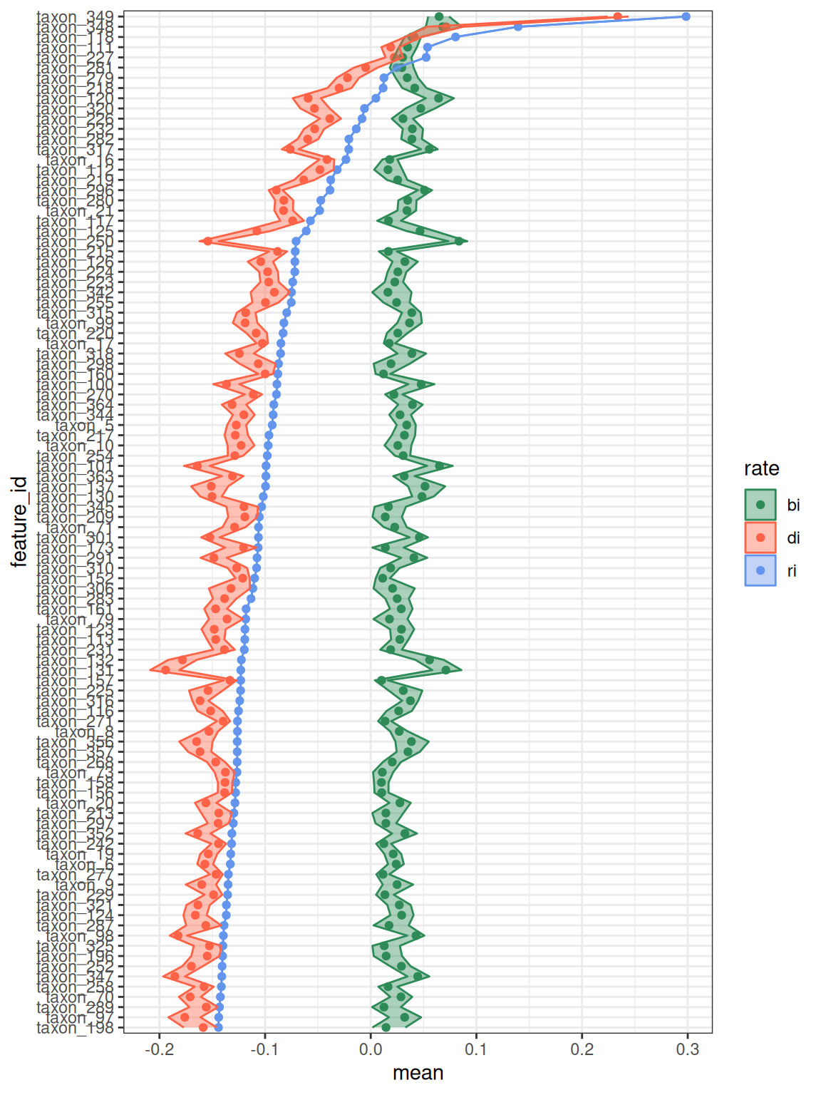

Figure 2: Growth values for the top 100 features showing birth and death rates with 90% confidence intervals.

When growth cannot be calculated

There are a few cases where growth cannot be calculated or the results can be non-sensical. Some cases result in the entire feature being unusable, while other cases just remove specific resamples for that feature while using the remaining resamples where possible. Understanding these edge cases is important for interpreting your results.

No time zero data

As noted in the warning when we ran get_N_total_it() above, taxon_194 has zero abundance at time zero. Therefore, the growth rate cannot be calculated because any change in abundance would be considered infinite growth. The intermediate values for these features can be found in the get_growth_data() function, but the feature will be omitted entirely from the summarize_growth_values() data.

Negative EAF values

This is related to the warning we received when running run_growth_calculations() stating there were 31862 resamplings that have “negative EAF values”. While negative EAF values can be common due to noise, it doesn’t make sense when calculating \(N_{LIGHTit}\) and \(N_{HEAVYit}\) values. This happens because \(N_{LIGHTit}\) gets calculated to actually have more copies than \(N_{TOTALit}\), which is impossible, and therefore \(N_{HEAVYit}\) will be a negative number of copies, which is also impossible. Table 6 shows examples from the q@growth$negative_labeled dataframe for taxon_1 explaining the reasoning. Z (equation 4 from Hungate et al. 2015⁴) is the difference between the labeled and unlabeled WAD value, so when Z is negative, it indicates the WAD values were lower for the labeled fractions, likely due to noise in the SIP process.

q@growth$negative_labeled |> 
  filter(feature_id == "taxon_1") |>
  select(feature_id, N_total_it, resample, Z, EAF, N_light_it, N_heavy_it)

Table 6: First few rows for taxon_1 showing negative EAF values and resulting negative N_heavy_it values.

feature_id	N_total_it	resample	Z	EAF	N_light_it	N_heavy_it
taxon_1	148586025	40	-0.0020331	-0.0309272	153190583	-4604557.9
taxon_1	148586025	56	-0.0023248	-0.0353985	153856294	-5270268.8
taxon_1	148586025	80	-0.0001851	-0.0028122	149004712	-418686.2
taxon_1	148586025	144	-0.0027846	-0.0422962	154883248	-6297222.6
taxon_1	148586025	145	-0.0003687	-0.0056138	149421834	-835808.9
taxon_1	148586025	290	-0.0007288	-0.0110860	150236552	-1650526.9

taxon_1 had a total of 28 resamplings fall into this category, but the remaining 972 were successful. This number is reflected in the successes column of summarize_growth_values().

summarize_growth_values(q, confidence = 0.9) |>
  filter(feature_id == "taxon_1") |>
  select(feature_id, successes)
#> Confidence level = 0.9
#> # A tibble: 1 × 2
#>   feature_id successes
#>   <chr>          <int>
#> 1 taxon_1          972

As long as a reasonable proportion of resamplings are successful (e.g., > 90%), the growth estimates are generally reliable. Features with very low success rates should be inspected more carefully or excluded from downstream analysis.

Conclusion

The growth workflow in qSIP2 extends the standard EAF calculations to estimate birth and death rates of individual features over time. By combining EAF values with quantitative abundance data at multiple timepoints, we can partition net community changes into their component processes — revealing whether features are actively growing, dying, or both.

Key points to remember:

• Growth analysis requires three additional columns in the source data: timepoint, total_abundance, and volume
• The workflow follows the same pattern as the standard qSIP workflow: filter, resample, calculate EAF, then add growth calculations
• Time zero abundances must be calculated using get_N_total_it() on the original unfiltered object
• Negative EAF values and missing time zero data can cause resampling failures, but as long as most resamples succeed the estimates remain robust
• The successes column in summarize_growth_values() indicates reliability of each feature’s growth estimate

Once you have growth results, you can use them to identify which features are responding to your experimental treatments by comparing birth and death rates across conditions.